Poland's Electricity Demand: What Temperature and Ramps Tell Us About System Stress
Electricity demand in Poland follows a clear temperature curve with a comfort minimum around 19°C. But peak load is only half the story — residual-load ramps exceeding 4 GW per hour reveal where real system flexibility is tested.
On Monday, January 12, 2026, Poland’s power system had to add more than 4 GW of dispatchable output in a single hour — between 05:15 and 06:15 — during already tight morning conditions. The peak demand that day was unremarkable. The ramp was not.
That distinction — between how much power the system needs and how fast it needs to change — is underappreciated. I see it in model after model: demand forecasts that nail the peak but ignore the ramp, capacity assessments that ask “do we have enough?” without asking “can we move fast enough?” Both questions matter. They test different things.
Temperature sets the daily playing field
I plotted weekday electricity demand in Poland against average 2-metre air temperature, split by time of day. Each dot is one hour.
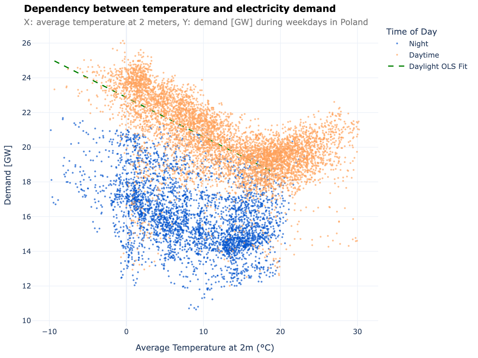
The scatter reveals a remarkably clean structure.
Daytime demand (orange) sits consistently 3–5 GW above nighttime demand (blue) across the entire temperature range. Commercial and industrial activity, lighting, and human routines create a higher baseline during the day. The consistency of this gap is what makes me confident these two regimes should always be modelled separately. Mixing them adds noise that obscures the temperature signal.
Both curves bottom out around 19°C. I call this the “comfort minimum” — the temperature where heating has switched off but cooling has not yet kicked in. It is not a hard threshold; it reflects the aggregate behaviour of millions of buildings and thermostats. But it is remarkably stable in the data, and it gives me a clean anchor for separating weather-driven load from structural baseload.
Below 19°C, the heating regime takes over. The relationship is close to linear: each 1°C drop is associated with roughly 0.23 GW of additional daytime demand. Over a 20-degree swing from mild autumn to deep winter, that adds up to 4–5 GW of extra load — a significant share of Poland’s total system capacity.
Above 19°C, demand starts climbing again as cooling loads increase. The cooling tail is less steep than the heating side in Poland — unlike southern European markets where air conditioning dominates — but it is visible and growing. As heat waves become more frequent and AC penetration rises, this right-hand side of the curve will steepen.
The coldest days in 2025 drove demand above 26 GW — with the annual peak recorded on November 24. On the hot end, the upward bend is gentler for now. But the structural trend toward higher cooling demand means summer peaks will become a more serious planning concern in the coming years.
Why this matters
If you are forecasting load, prices, or renewable capture factors, temperature is not just another input feature — it sets the daily playing field. A 5°C cold snap does not just shift demand up; it changes the merit order position of marginal generators, tightens reserve margins, and alters how much room the system has to absorb renewable output.
The comfort minimum is particularly useful as a reference point. A “mild winter” and a “cold winter” are not abstract labels — they translate into specific GW differences through the temperature-demand slope.
Peak demand is a capacity question — ramps are a flexibility question
Demand levels tell you how much generation the system needs. They do not tell you how fast the system needs to respond.
Residual load — total demand minus wind and solar generation — represents what the dispatchable fleet must cover. The ramp is how quickly that residual load changes from one hour to the next. A 2 GW upward ramp means 2 GW of additional dispatchable capacity online within an hour. The faster the ramp, the more it tests start times, ramping rates, and reserve margins.
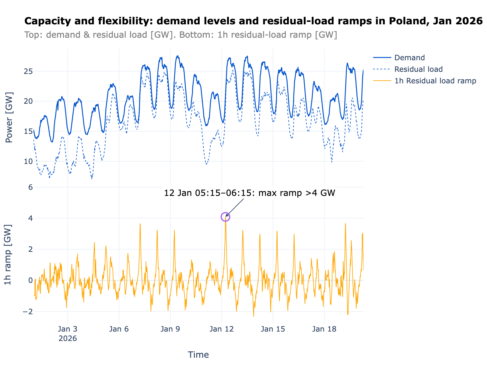
The daily rhythm is visible: demand ramps up sharply each morning as the country wakes up and industrial loads switch on, then falls through the evening. But the magnitude of some of these ramps is what matters.
That January 12 event — over 4 GW in a single hour — happened during already tight morning conditions. Even though the absolute demand level was manageable, the ramp tested whether enough fast-start units were already online, whether sufficient reserves were scheduled, and whether operational margins could absorb the surge during hours when solar output was absent and demand was still climbing. A system that looks adequate on paper at 8am can still be stressed at 6am if it cannot ramp fast enough to get there.
These 4 GW+ ramp events are not daily, but they are not rare either. And as renewable penetration grows, I expect them to become more frequent. The reason is straightforward: residual-load ramps are driven not just by demand changes but by the rate at which solar output appears and disappears. On a clear winter morning, solar can ramp from zero to several GW within two hours. On a cloudy morning, it barely shows up. The difference creates additional volatility that the dispatchable fleet must absorb.
Two halves of the same problem
Temperature and ramps describe two complementary aspects of system stress.
Temperature tells you the level — how much total demand the system faces. It is a capacity question: do I have enough generation and import capacity to meet peak winter demand when temperatures drop below -10°C?
Ramps tell you the dynamics — how fast the system needs to respond. It is a flexibility question: can the fleet ramp fast enough to cover a 4 GW morning surge when renewable output is volatile and uncertain?
A system can be adequate on capacity and still fail on flexibility. I think Poland’s January 2026 data makes this case clearly: a month with manageable peak demand that still produced individual hours capable of stressing the system. As the energy mix shifts toward higher shares of variable renewables — a transition I have been tracking through my analyses of residual load and prices and renewable capture factors — the flexibility dimension will only grow in importance.
The practical takeaway: demand forecasts should include not just the level but the ramp. Temperature sensitivity gives you the first. Decomposing residual load gives you the second. You need both to understand where system stress actually comes from.
More posts
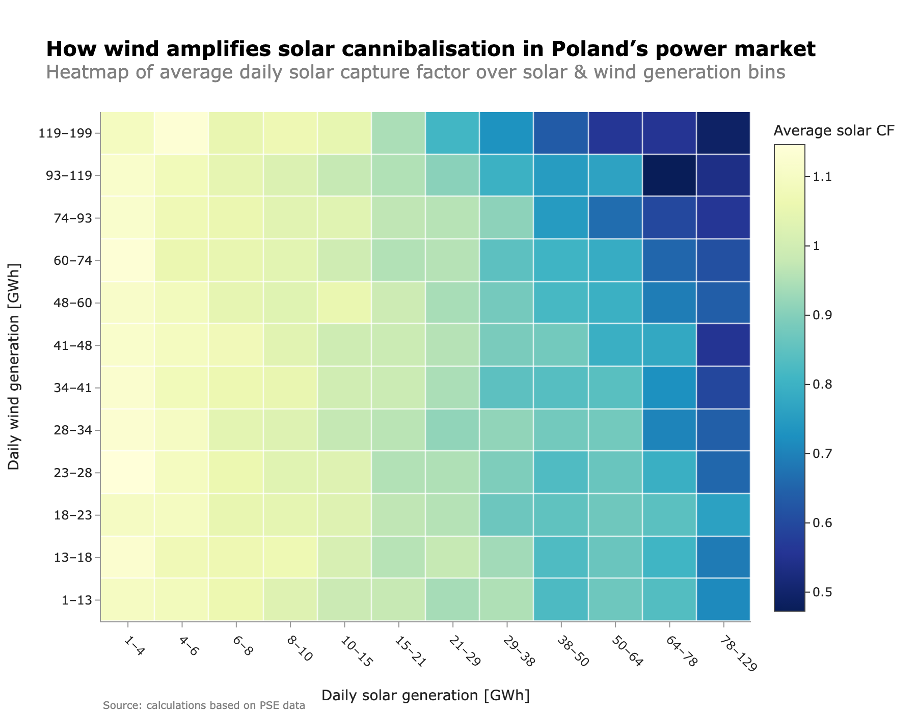
Solar Cannibalization in Poland: How Capture Factors Erode as Renewables Scale
Solar capture factors in Poland have fallen below 50% in peak months — and the decline accelerates with penetration. A two-dimensional look at how both solar volume and wind output shape PV revenues, and what the curve ahead looks like.
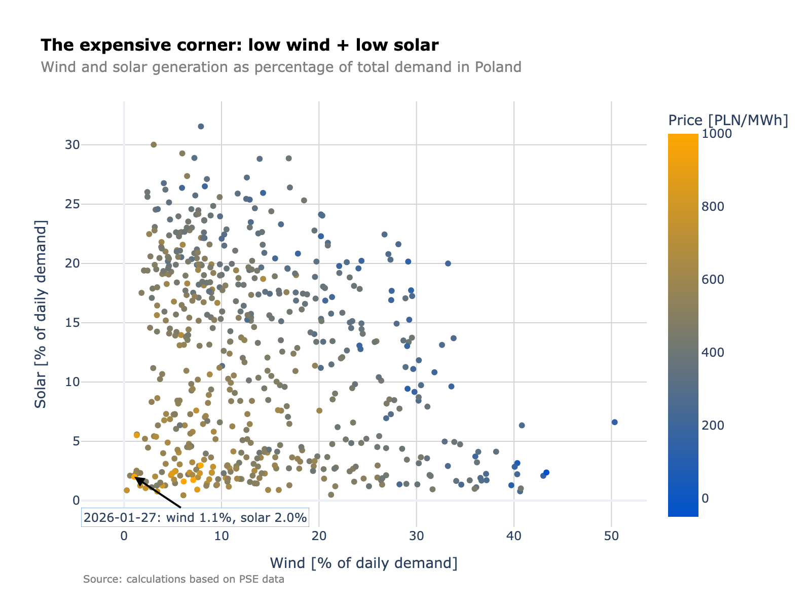
When Wind and Sun Both Disappear: Joint Renewable Scarcity and Prices in Poland
Days with low wind and low solar are not rare — they are a recurring regime in Poland that drives the highest wholesale prices. Residual load, not total demand, is the real scarcity signal.
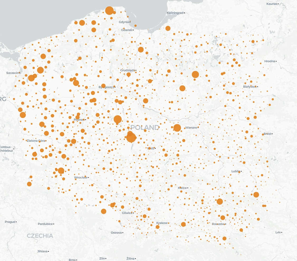
Poland's Solar Map: Where Capacity Is Concentrating and Why Location Matters
Poland now has a nationwide solar fleet — but capacity is clustering, not spreading evenly. The top 1% of installations account for 28% of capacity. Geographic concentration drives correlated output, congestion risk, and curtailment exposure.