
·
How Residual Load Shapes Wholesale Electricity Prices in Poland
Residual load — demand minus wind and solar — is the single best lens on Poland wholesale power prices from 2020 to 2025. Year-by-year evolution, the rise of negative prices, and the month × hour price-sensitivity surface that anchors what-if analysis.
TL;DR
- Residual load — demand minus wind and solar — explains a substantial share of hourly wholesale price variance in Poland. Its explanatory power dropped during the 2021–2022 fuel crisis (R² down to 0.2) and has recovered to 0.53 in 2025 as gas, coal, and carbon inputs stabilised.
- The relationship is convex and state-dependent. Marginal price sensitivity ranges from under 4 PLN/MWh/GW at summer night lows to over 196 PLN/MWh/GW during evening peaks — a 49× spread. A single elasticity for Poland is misleading; the month × hour surface is the right representation.
- Below roughly 10 GW of residual load, prices increasingly clear at zero or negative values. Poland recorded 204 negative-price hours in 2024 and 356 in 2025.
In this post I take a simple, practical look at how one metric – residual load – helps explain Poland’s power prices over the last few years.
No single variable tells the whole story in a market that has gone through a fuel crisis, fast renewables build‑out and regulatory changes. But residual load (demand minus renewables) turns out to be a very useful starting point — and the foundation that the rest of the analyses in this series.
I focus on straightforward visuals: scatter plots of residual load versus market prices (PLN/MWh) from the Polish day‑ahead market, based on data published by PSE, year by year from 2020 to 2025. The goal is to see what we can already learn from the charts before moving on to more detailed “what‑if” analysis in the next step.
What is residual load?
Residual load is the portion of demand that must be covered by dispatchable generators after subtracting variable renewables (mainly wind and solar):
Residual load = Total demand − Wind − Solar
Residual load is a very useful metric for understanding price formation. It directly links the merit order to prices: the higher the residual load, the more capacity has to be brought online, typically from more expensive plants. It also implicitly captures many structural changes in the system — renewables build‑out, demand trends, and changes in thermal fleet availability. And it is straightforward to use in “what‑if” terms: for example, we can ask what happens to prices if residual load is 2 GW lower because more PV is added to the system, or how prices respond when 1 GW of BESS shifts load and discharge across hours.
Residual load vs wholesale price in Poland, 2020–2025
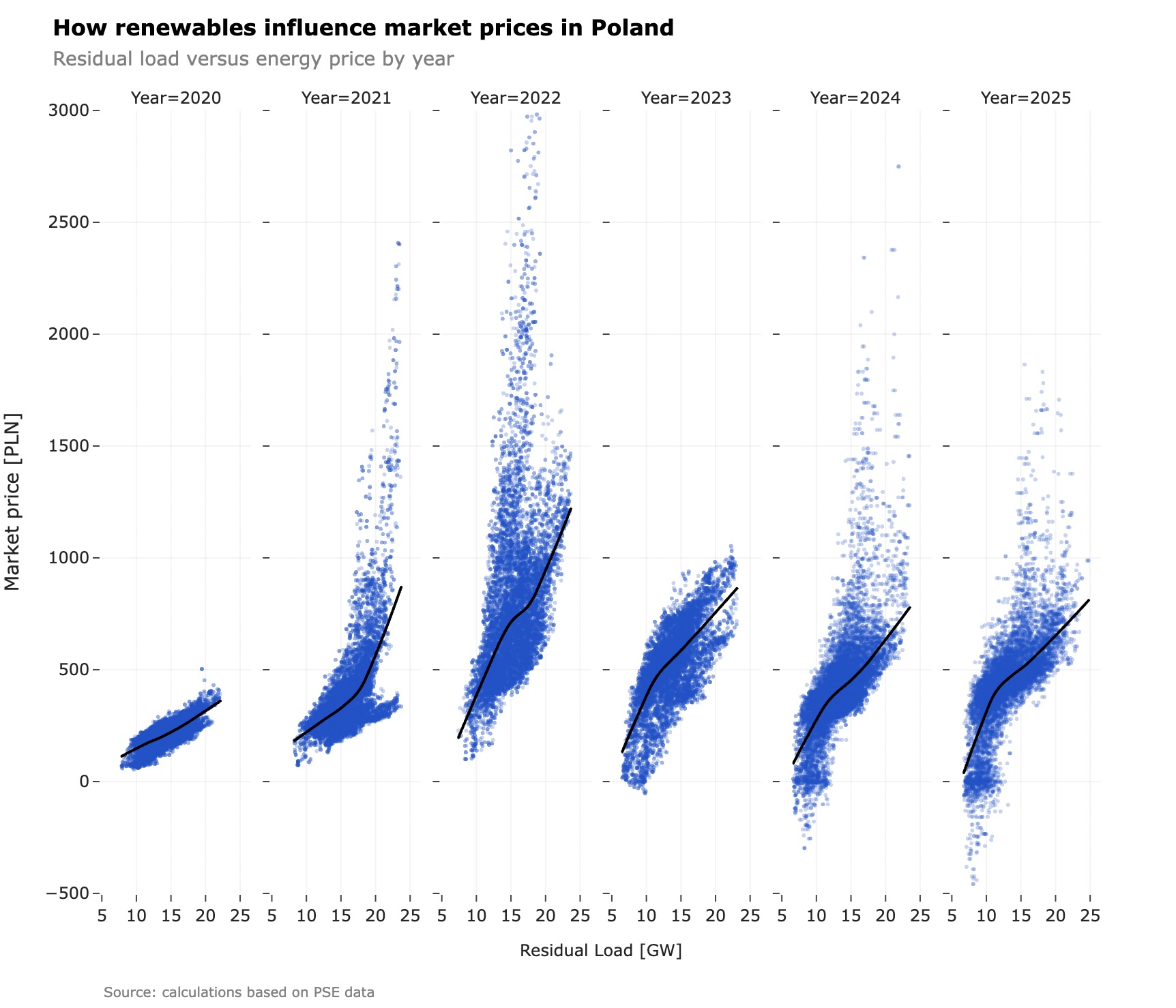
The figure above compares hourly market prices (PLN/MWh) against residual load (GW) for each year from 2020 to 2025. Each point is an hour; the black line is a smoothed trend for that year. Even without any modelling, the scatter already spells out how the merit order shows up in prices.
Across years, the whole curve shifts. For a given level of residual load, prices in 2021 and especially 2022 sit well above other years – the fuel crisis in picture form, as higher gas and coal prices plus high carbon costs lifted the entire merit order. From 2023 onwards the curves move back down: the same 15 GW of residual load that implied very high prices in 2022 corresponds to much more moderate prices by 2024–2025 as input costs ease and more renewables enter the system.
Another notable feature is how the shape of the curve evolves over time. In 2020 the dependency is relatively linear, with prices rising steadily as residual load increases. Years 2021 and 2022 show increasing curvature, with prices escalating more sharply at higher residual loads due to heightened fuel costs. The curve is convex – relatively flat at low residual loads and gets steeper as residual load increases, reflecting the growing impact of expensive peaking units during high demand periods. This is particularly evident in 2021.
The goodness-of-fit also moves over time. Fitting a smooth curve year by year and recording R² together with a few headline statistics:
| Year | R² (smoothed fit) | Mean price (PLN/MWh) | Hours at price ≤ 0 | Installed RES (GW) |
|---|---|---|---|---|
| 2020 | 0.59 | 208.6 | 0 | 10.4 |
| 2021 | 0.39 | 398.1 | 0 | 14.8 |
| 2022 | 0.2 | 787.3 | 0 | 20.4 |
| 2023 | 0.53 | 510.7 | 33 | 26.5 |
| 2024 | 0.45 | 415 | 204 | 31.3 |
| 2025 | 0.53 | 441.9 | 356 | 34.9 |
The explanatory power of residual load alone drops during the fuel crisis – as gas, coal and carbon prices became the dominant source of short-term price variance – and recovers once input costs stabilise. In 2025 residual load is once again the dominant single explanatory variable. The practical implication for anyone calibrating a price model: residual load is necessary, sufficient most of the time, and insufficient during regime breaks. Layering in fuel prices and carbon is a second-order correction, not a first-order rebuild.
The rise of zero and negative prices
From 2024, a new feature appears at the low‑load end: more hours clear at zero or negative prices, and the trend line develops a visible downward bend around roughly 10 GW of residual load. Together, these points show that risk in the market has become two‑sided – very high prices when residual load is large and the system is tight, and very low or negative prices when residual load is small and inflexibility dominates. By 2025 this is no longer a curiosity but a regular operating condition, with 356 hours of negative prices recorded over the year.
Growing wind and solar push more hours into very low residual load territory. At the same time a large block of must‑run or low‑flex capacity (technical minima, CHP, long‑ramp thermal units) limits downward adjustment. When residual load sinks below this flexible threshold the clearing price has to fall.
This is the same dynamic that drives PV capture factors lower as solar capacity scales – I cover the revenue side of that story in Poland’s solar generation boom and the decline in PV capture factor.
Seasonal view of residual load
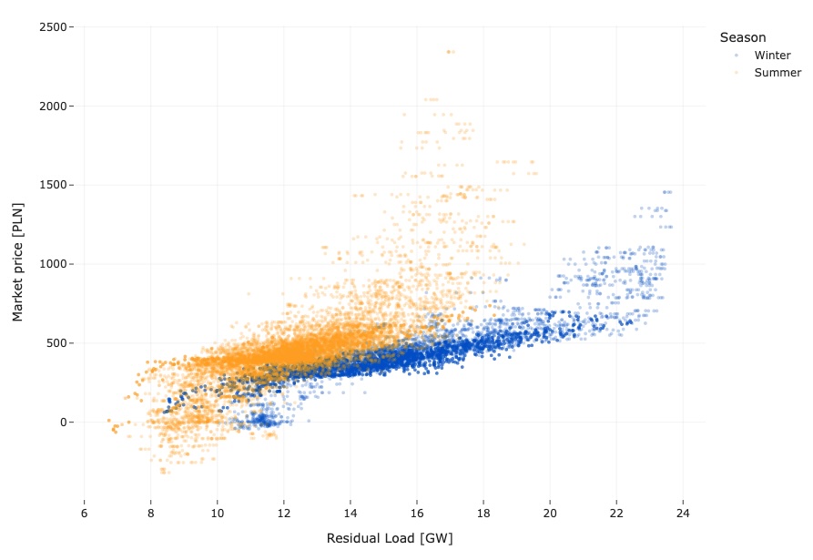
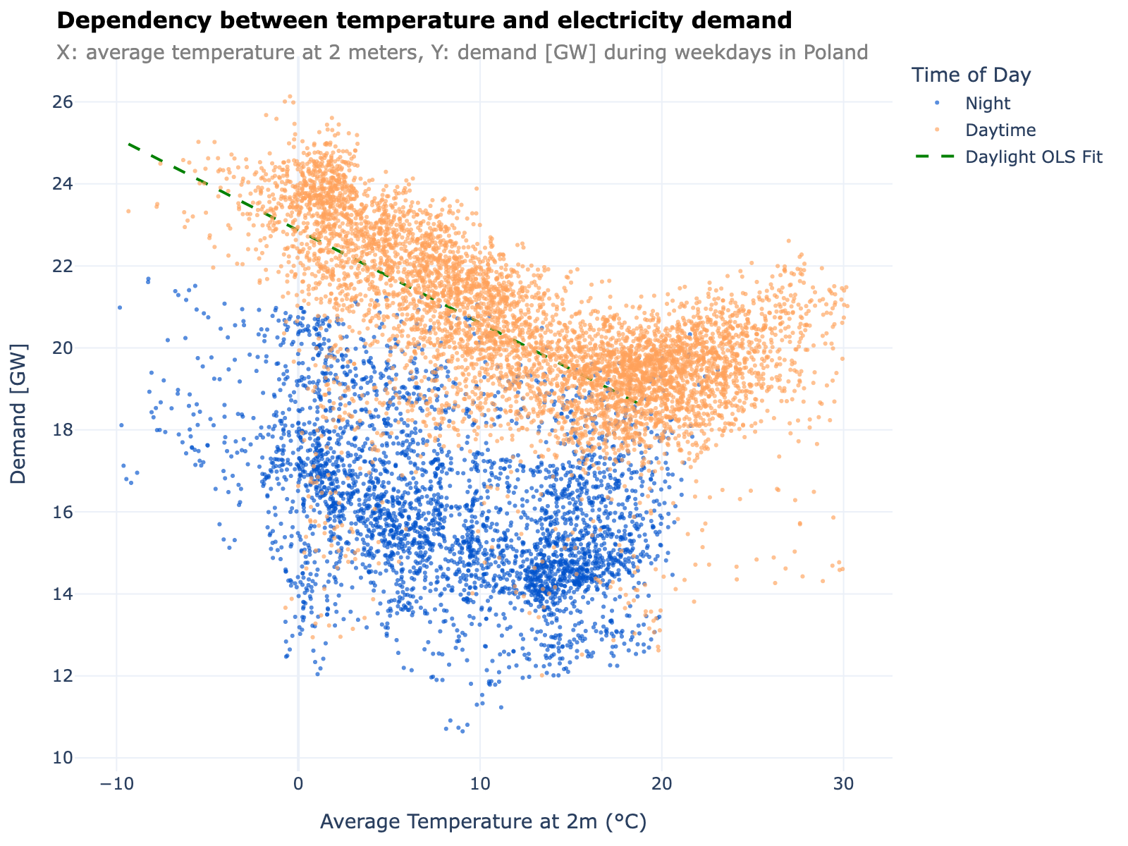
Looking at the relationship by season adds another layer of detail. Winter operates over a wider residual-load range, with P99 reaching approximately 23.1 GW as heating demand adds several GW on cold days. The temperature mechanics behind this winter ramp – including the segmented heating slope of −0.194 GW/°C measured around a comfort minimum of 16.5°C – are covered in Poland’s electricity demand: what temperature and ramps tell us about system stress.
Summer residual loads typically stay below 19.2 GW but deliver higher prices for the same residual load. The summer curve sits visibly above winter at equivalent load levels, driven by tighter reserve margins during maintenance outages, a thinner thermal fleet, and hotter cooling water constraining some units. Summer also shows more hours with negative prices and more extreme spikes, with a visibly steeper residual-load/price slope.
Why this matters for “what-if” analysis
This evolving residual-load/price relationship is more than just a nice chart – it’s a practical tool.
If we can quantify the marginal sensitivity (PLN/MWh per GW) by season and hour, we can estimate renewable impacts (e.g. +2 GW PV deepening midday summer lows), value demand‑side shifts (lowering residual load in targeted blocks), and compare strategic portfolios: more batteries clipping peaks and possibly dampening low/negative episodes, or thermal fleet changes that alter steepness at high loads.
Residual-load price sensitivity by month and hour
To move from “what happened” to “what if”, we also need to know how much prices react to a small change in residual load at different times of the year and day. Here I map marginal price sensitivity (PLN/MWh change per 1 GW residual load shift) on a month × hour heatmap.
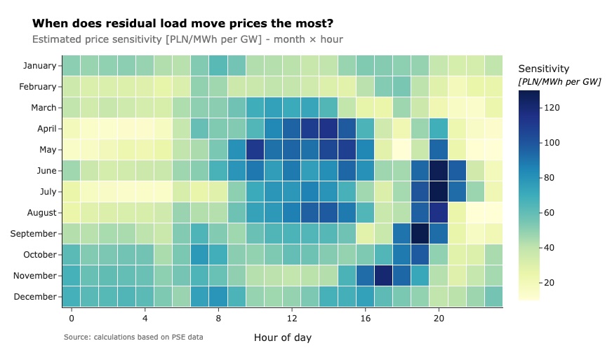
Looking at the heatmap, a few patterns stand out. Around the midday “solar dip” in residual load, even a small upward shift (less PV or a bit more demand) quickly pulls higher‑cost units onto the margin – the dark core in the middle of the plot, where sensitivity reaches roughly 140 PLN/MWh per GW in April. Put differently, a bit more solar generation in those hours quickly pushes prices down. At high demand in the morning and especially in the evening peak, sensitivity spikes again: extra residual load there steepens the curve fastest, peaking at around 196 PLN/MWh per GW. By contrast, nights – particularly in summer – look relatively flat.
The ratio between the most and least sensitive cells is on the order of 49×, which is why a single price elasticity for “Poland” is misleading. The same 1 GW of incremental PV or BESS discharge can move price by an order of magnitude more in one cell of the surface than in another.
The key insight is that the residual load impact is non‑linear: the more extreme the price level, the more sensitive it becomes to additional load. That convexity is the merit order in action — climbing the stack not only costs more per MW, the slope itself steepens at higher utilisation.
Implications.
A ±1 GW shift matters most in the midday trough and the evening peak; with rising RES penetration I expect those swing zones to widen and deepen. The sensitivity matrix also lets us compare +1 GW wind (flatter diurnal profile) vs +1 GW solar (midday‑heavy) and see how each reshapes the slope and volatility of the price curve.
From a business perspective, the heatmap shows when the market is most price‑sensitive to changes in residual load. That matters whenever new capacity is added or existing capacity is shifted, because those changes will move residual load and, in turn, reshape prices hour by hour. In rough terms, price change follows residual load change scaled by the sensitivity in each month and hour.
This has direct consequences for capture factors and revenues. Adding solar or wind into hours with high sensitivity is more likely to drag prices down and compress capture prices, especially around the midday trough; adding into flatter parts of the heatmap has a softer effect on price levels and on realised revenues. The same logic applies to storage and demand response: shifting load away from high‑sensitivity hours, or discharging into them, can have an outsized impact on both price levels and on the daily price spread that batteries monetise. You can read more about capture-price dynamics in Poland’s solar generation boom and the decline in PV capture factor and in my live capture factor dashboard.
Methodology and data
Data sources. Hourly demand, wind, and solar generation from PSE, 2020–2025. Hourly day-ahead wholesale prices (RCE, PLN/MWh) from the same source.
Residual load. Defined as Demand − Wind − Solar at hourly resolution. No correction for
imports/exports or for prosumer self-consumption.
Year-by-year fit. LOWESS smoother (bandwidth 0.3) fitted separately within each calendar year. R² computed as 1 − SS_residual / SS_total against the smoothed prediction.
Sensitivity surface. For each of the 12 × 24 = 288 month × hour cells, I fit a local regression of price on residual load across all years pooled and evaluate the local slope at the cell’s mean residual load. This gives the PLN/MWh per GW surface shown in Figure 3.
Caveats. Residual load is a strong but incomplete predictor — fuel prices, carbon, neighbouring markets and unit outages explain additional variance, particularly during regime breaks like 2022.
Get new posts by email
Empirical analysis of Poland's power markets and the energy transition, delivered when new posts go live. No spam.
More posts
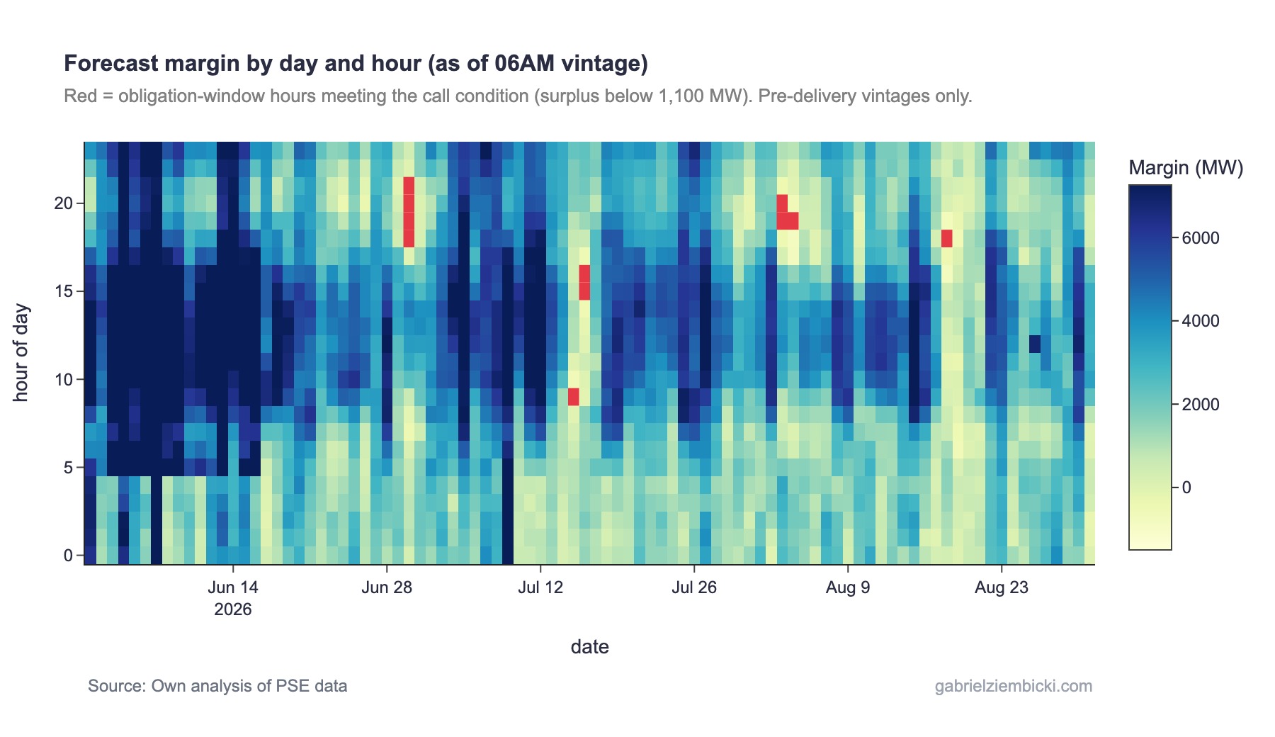
What actually happens when Poland triggers a capacity market call
Poland's capacity market (rynek mocy) was called three times in the summer of 2026 — more than in the previous five years combined. I reconstruct the capacity market call trigger PSE publishes, compare the three call days with similarly stressed days on which no call was declared, and show which factors actually drove the margin shortfall.
How much do Polish renewables actually earn? Solar and wind capture prices explained
What a MWh of Polish solar and wind actually earns, measured through capture price and capture factor. This post tracks how those numbers have moved since 2020, why wind and solar diverge, and what it means for project economics.
Poland's electricity demand: what temperature and ramps tell us about system stress
Demand in Poland follows a clean two-regime temperature curve with a comfort minimum at 16.5°C and a heating-side slope of 0.213 GW/°C. Residual-load P99 1-hour ramps reached 3.22 GW in 2024–2025 and will likely grow further with PV. A quantitative look at both.