Poland's electricity demand: what temperature and ramps tell us about system stress

TL;DR

• Polish weekday demand follows a piecewise-linear temperature curve with a comfort minimum at around 16.5°C. There is 0.194 GW increase per 1°C drop below that point, and 0.086 GW increase per 1°C rise above that temperature. Day/night baseline gap is around 4.2 GW. These three numbers explain 57% of variance in demand on weekdays.
• P99 of 1-hour residual-load ramps reached 3.22 GW in 2024–2025 — driven primarily by solar output volatility and by changes in underlying demand dynamics.

On Monday, January 12, 2026, Poland’s power system added more than 4 GW of dispatchable output in a single hour — between 05:15 and 06:15.

Capacity adequacy assessments ask “do we have enough?” without asking “can we move fast enough?” Both questions matter, and they test different parts of the fleet.

This post does two things. First, it fits a piecewise-linear regression of demand on temperature and reports the slopes with uncertainty. Second, it pulls apart the distribution of 1-hour residual-load ramps, focusing on the tail, and shows how the tail has evolved.

Temperature sets the level — in two regimes

Weekday electricity demand plotted against simple average 2-meter air temperature (probably a population-weighted average would work even better here), split by time of day:

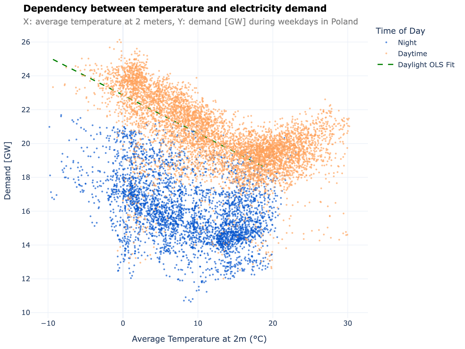
The structure is clean enough that I can summarise it in four numbers. I fit a segmented regression of the form:

Demand_h = β₀ + β_day·Day_h + β_heat·max(16.5 − T_h, 0) + β_cool·max(T_h − 16.5, 0) + ε_h

where Day_h is a daytime indicator (07:00–22:00 CET) and T_h is the simple-average ERA5 2m temperature across grid cells over Poland. Results over 2024–2025 (9,461 weekday hourly observations):

Parameter	Estimate	Interpretation
Day/night gap (β_day)	4.22 GW	Structural gap from activity patterns
Heating slope (β_heat)	−0.194 GW/°C	Each 1°C below 16.5°C raises demand by 0.194 GW
Cooling slope (β_cool)	+0.086 GW/°C	Each 1°C above 16.5°C raises demand by 0.086 GW
Breakpoint	16.5°C	Data-driven estimate; clusters tightly
R² (within-weekday)	0.569	Share of variance explained

Three things to highlight.

The breakpoint at 16.5°C is not imposed — it is the temperature the data itself points to as the elbow of the curve — obtained by re-running the least-squares fit at different candidate breakpoints and keeping the one with the best fit. It gives a clean anchor for separating weather-driven load from structural baseload.

The heating slope is significantly steeper than the cooling slope — roughly 2.2 times larger. The 17.5°C swing from mild autumn (≈16.5°C, near the comfort minimum) to deep winter (≈−1°C) translates to roughly 3–4 GW of additional load via the heating slope alone.

Ramps: level plus dynamics

Demand levels tell you what the dispatchable fleet must deliver. Ramps tell you how fast. The relevant quantity is residual-load ramp — the hour-to-hour change in (demand − wind − solar):

residual_load = demand - wind - solar
ramp_1h = residual_load.diff(4)                # GW change in 4 quarter-hours
p99_up = ramp_1h[ramp_1h > 0].quantile(0.99)   # worst upward ramp hour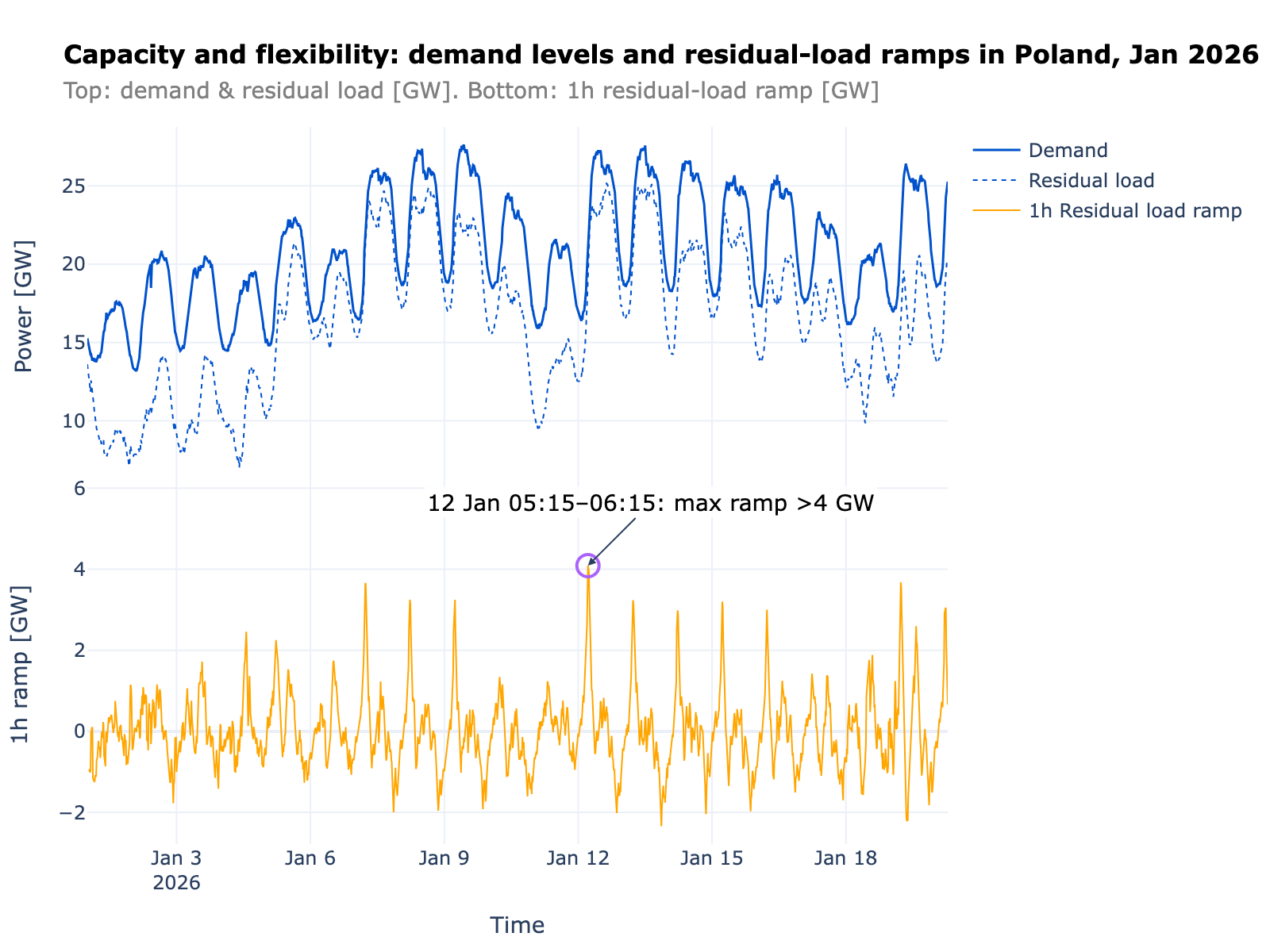

Let’s have a look at the distributiion:

Quantile (absolute 1h ramp)	Demand only	Residual load	Gap
P50	0.45 GW	0.70 GW	+0.25
P95	1.77 GW	2.44 GW	+0.68
P99	2.76 GW	3.22 GW	+0.46
Max observed	3.86 GW	5.96 GW	—

Three patterns I want to highlight.

The tail gap between demand ramps and residual-load ramps is significant - at the 99th percentile, residual-load ramps are 17% larger than demand-only ramps — meaning that when the dispatchable fleet faces its hardest hours, some of the difficulty comes from what renewables are doing, not only from the demand behaviour.

Decomposing the largest ramps confirms it. On the 50 worst upward residual-load ramp events in 2024–2025, the contributions were roughly:

Driver	Share of ramp magnitude
Solar output falling	69%
Wind output falling	5%
Demand rising	25%

Solar dominates the tail on the upward side: at sunset, PV output falls from several GW back to near-zero within roughly two hours. On the downward side — the largest negative ramps, when the system is suddenly oversupplied. The tail increased in 2025 compared to 2025. Rolling P99 of residual-load ramps by year:

Year	P99 upward ramp (GW/h)	P99 downward ramp (GW/h)	Installed PV (GW)
2024	3.17	2.46	~21
2025	3.42	2.87	~23

Methodology and data

Data sources. Hourly demand, wind, and solar generation from PSE, 2024–2025. Hour-ending convention; timestamps aligned to local civil time. Temperature from ERA5 2m air temperature, hourly, aggregated to a national value by simple averaging across grid cells over Poland. A population- or industry-load-weighted mean would likely fit demand better; the simple-average choice is conservative and easier to reproduce.

Segmented regression. Piecewise linear fit with breakpoint estimated via grid search over 12–20°C in 0.5°C steps, selecting the breakpoint that minimises the residual sum of squares. Heteroskedasticity-consistent (HC3) standard errors. Day indicator covers 07:00–22:00 CET. Weekdays only (9,461 observations); separate fits for weekends gave qualitatively identical slopes with different intercepts (not shown).

Ramp definitions. 1-hour ramp = residual_load(t) − residual_load(t−4). Separate P99s for positive and negative ramps, computed within-year to track tail evolution over time.

Decomposition of largest ramps. For each of the top 50 upward residual-load ramps, I decompose the magnitude into demand, −wind, and −solar components (additive by construction) and report the sample mean of each contribution’s share.

Cold-tail demand calculations. Use the fitted segmented regression evaluated at the P99 cold daily temperature from the ERA5 series.

Caveats. The cooling-slope estimate (+0.086 GW/°C) is based on a short time series (2024–2025) and should be treated as an early-stage signal; a longer historical baseline would improve this estimate considerably.

---